Transmission Lines and Its Equations

Energy can be transmitted either by radiation of free electromagnetic waves or can be varied in various conductor arrangement known as Transmission Lines. Transmission line is a conductive method of guiding electric energy from one place to another. They act as a link between antenna and transmitter or receiver. They are also used as circuit elements i.e. like resistor, inductor or capacitor etc. Basically there are four types of transmission lines.

Types of Transmission Lines

Two-Wire Line

• Two parallel conductors separated by air or an insulating medium. Common in low-frequency RF systems, telegraph lines, and antenna feeders. Simple construction, low cost. Prone to radiation losses, interference, and noise pickup.

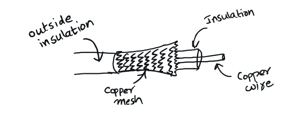
Coaxial Cable

• Consists of a central conductor surrounded by an insulating dielectric, a metallic shield, and an outer insulating jacket. Widely used in cable TV, internet connections, and RF systems. Excellent shielding reduces interference, ideal for high-frequency signals. Bulkier and more expensive than two-wire lines.

Microstrip Line

• A flat conductor strip printed on a dielectric substrate with a ground plane on the opposite side. Used in microwave circuits, antennas, and PCB designs. Compact, easily integrated into PCBs. Higher radiation loss at higher frequencies.

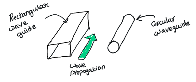
Waveguide

• A hollow metallic tube that guides electromagnetic waves. Used for microwave and millimeter-wave communications, radar systems. Very low loss at high frequencies, ideal for power transmission in microwave bands. Expensive, bulky, and requires precision manufacturing.

Equivalent Circuit of a Transmission Line

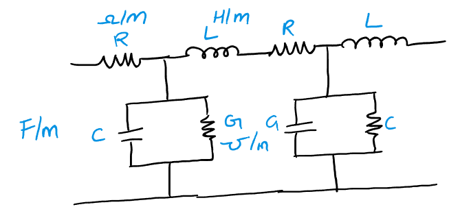
The primary constants of a transmission line are fundamental parameters that define its electrical behavior. These are:

1. Resistance (R)
   • Measured in ohms per unit length (Ω/m).
   • Represents the conductor’s resistance, causing power loss as heat.
   • Higher at lower frequencies due to DC resistance effects.
2. Inductance (L)
   • Measured in henries per unit length (H/m).
   • Represents magnetic energy storage due to current flow.
   • Influences signal delay and impedance.
3. Capacitance (C)
   • Measured in farads per unit length (F/m).
   • Represents the electric field energy stored between conductors.
   • Affects signal distortion and propagation.
4. Conductance (G)
   • Measured in siemens per unit length (S/m).
   • Represents leakage current through the insulating material.
   • Higher values result in greater dielectric losses.

These constants impact signal attenuation, phase shift, and impedance, making them crucial for efficient transmission line design.

Transmission Line Equations

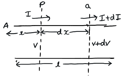
Step 1: Voltage Equation

The potential difference between two points is given by:
\[
V – (V + dV) = I (R + j\omega L) dx
\]

Simplifying,
\[
-dV = (R + j\omega L) I dx
\]

Dividing both sides by \( dx \),
\[
\frac{-dV}{dx} = (R + j\omega L) I \quad \text{(Equation 1)}
\]

---

Step 2: Current Equation

From Kirchhoff’s current law,
\[
I – (I + dI) = V (G + j\omega C) dx
\]

Simplifying,
\[
-dI = (G + j\omega C) V dx
\]

Dividing both sides by \( dx \),
\[
\frac{-dI}{dx} = (G + j\omega C) V \quad \text{(Equation 2)}
\]

---

Step 3: Deriving Second-Order Equations

Differentiating Equation 1:
\[
\frac{d}{dx} \left( \frac{dV}{dx} \right) = \frac{d}{dx} \left[ (R + j\omega L) I \right]
\]

Using Equation 2,
\[
\frac{d^2V}{dx^2} = (R + j\omega L)(G + j\omega C) V
\]

Similarly, differentiating Equation 2:
\[
\frac{d}{dx} \left( \frac{dI}{dx} \right) = \frac{d}{dx} \left[ (G + j\omega C) V \right]
\]

Using Equation 1,
\[
\frac{d^2I}{dx^2} = (R + j\omega L)(G + j\omega C) I
\]

---

Step 4: Final Form

Let
\[
\gamma^2 = (R + j\omega L)(G + j\omega C)
\]

Then,
\[
\frac{d^2V}{dx^2} = \gamma^2 V
\]

\[
\frac{d^2I}{dx^2} = \gamma^2 I
\]

Where \( \gamma \) is the **Propagation Constant**.

Equations (3) and (4) are the **differential equations of transmission lines**.

Solution of Transmission Line Equations

\[
V = ae^{px} + be^{-px}
\]
\[
I = ce^{px} + de^{-px}
\]

Where \(a\), \(b\), \(c\), and \(d\) are constants.

Hyperbolic Identity Substitution

\[
e^{px} = \cosh(px) + \sinh(px)
\]
\[
e^{-px} = \cosh(px) – \sinh(px)
\]

Modified Equations

\[
V = A \cosh(px) + B \sinh(px)
\]
\[
I = C \cosh(px) + D \sinh(px)
\]

Where:
– \( A = a + b \)
– \( B = a – b \)
– \( C = c + d \)
– \( D = c – d \)

Differentiation and Substitution

\[
-\frac{dV}{dx} = (R + j\omega L) I
\]
\[
-\frac{d}{dx} (A \cosh(px) + B \sinh(px)) = (R + j\omega L) I
\]
\[
-(Ap \sinh(px) + Bp \cosh(px)) = (R + j\omega L) I
\]

Substituting

\[
p = \sqrt{(R + j\omega L)(G + j\omega C)}
\]

\[
-\frac{G + j\omega C}{R + j\omega L} (A \sinh(px) + B \cosh(px)) = I
\]

Final Solution

\[
I = -\frac{1}{Z_0} (A \sinh(px) + B \cosh(px))
\]
\[
V = A \cosh(px) + B \sinh(px)
\]